In this project I worked on benchmarking a Deep Learning approach to mixed-illuminant whitebalance in comparison with analytical methods based on images from a polarization camera. In a 5 person team of media technology students at TH Köln, I was responsible for deploying a pre-trained Deep Learning model to our custom camera preprocessing pipeline, that was uniquely designed for the specific camera hardware.
This project showcases my abilities to
- work with a custom camera pipeline in Python,
- deploy a pre-trained Deep Learning model to a custom infrastructure,
- evaluate the performance of a Deep Learning model against analytical methods,
- work with image data and to preprocess it for Deep Learning applications efficiently,
- think analytically about the problem and to design a custom evaluation data set,
- understand complex math behind technical innovation and their contribution to domain-specific problems,
- work in a team and to communicate results effectively.
The Deep Learning part
For the whitebalance predictions, we used the Deep Neural Network from Mahmoud Afifi. I wrote a custom class, that holds this model and can be used in our node-based image pipeline. This pipeline is written in Python and uses OpenCV for image processing. It is used to preprocess the raw images from the camera, apply a color profile, and to apply the whitebalance correction to the images.
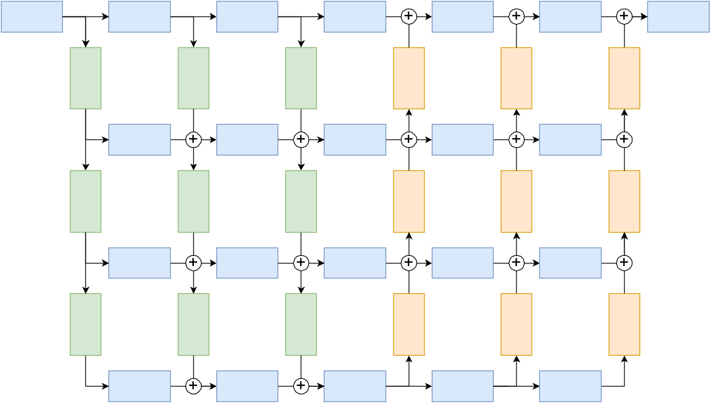
The DNN has learned to generate mappings for 5 predefined white balance settings, that are commonly used in photography. That makes it possible to use the net in a modified camera. The camera has to render every image with 5 predefined white balance settings no matter what the scene actual demands. The network then creates mappings to correct the white balance in post-processing. When learning about this architecture and how the authors trained it, I was really buffled how they instrumentalized the loss function to achieve visually pleasing results. The overall loss function is defined as
In this loss function,
To further improve the results, additional steps have been taken by Afifi et al.: Firstly a cross-channel softmax operator has been applied before loss calculation in order to avoid out-of-gamut-colors. In this step, the exponential function is applied to each element and the output is then normalized by dividing by the sum of all new values. Secondly, a regularization term is introduced to the loss function. Hereby, GridNet is trained to produce rather smoothed weighting maps opposed to perfectly accurate maps. This may be due to reasons of generalization as well as visual observation by the researchers. The regularization is applied with
with
Benchmarking experiments
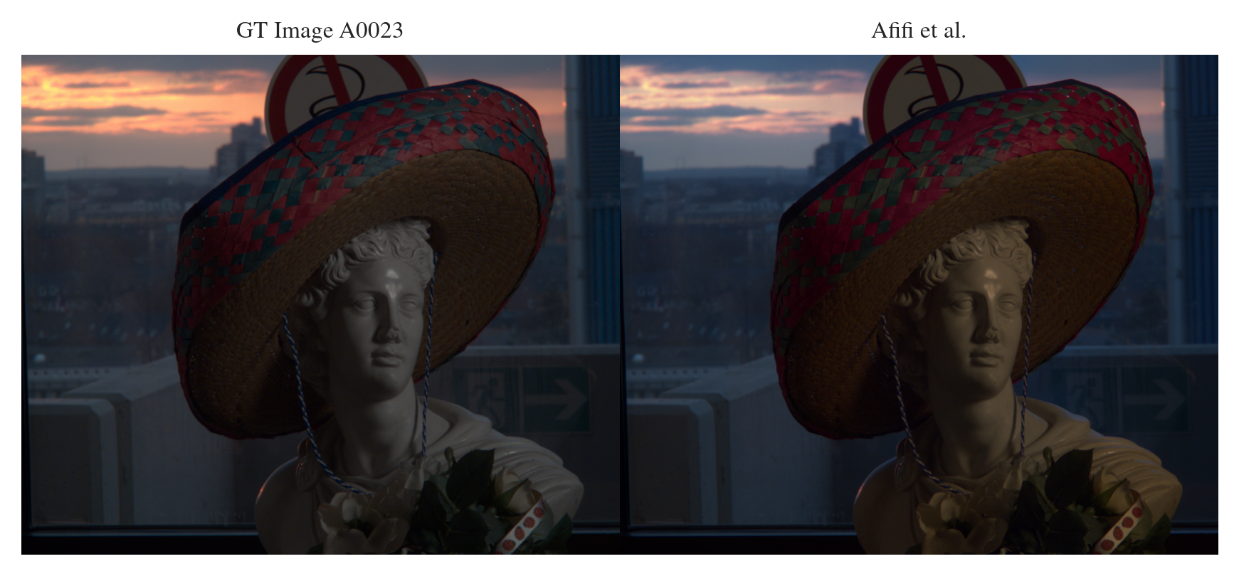
Now, to compare this Deep Learning approach with the analytical methods, we produced a unique evaluation data set, that is super hard to white balance. We photographed images with extreme mixed illuminant scenarios where two light sources of opposing color temperatures were lighting the scene or sometimes were even visible in the image. We then compared the results of the Deep Learning approach with the analytical methods based on the polarization camera images by employing error metrices.
Let’s see how the DNN works in one example of our benchmarking data set:
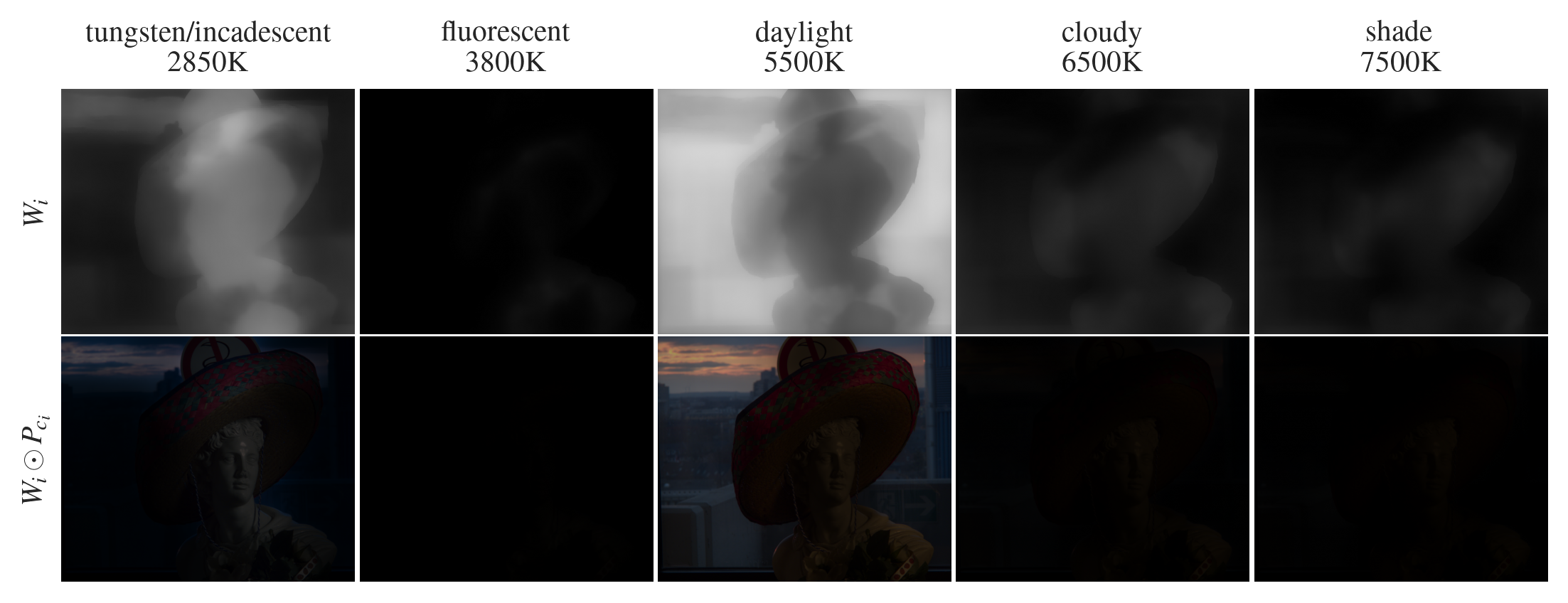
We can also inspect, what the DNN did under the hood by plotting the weighting maps and the Hadamard products of the weighting maps and the pre-rendered WB images:
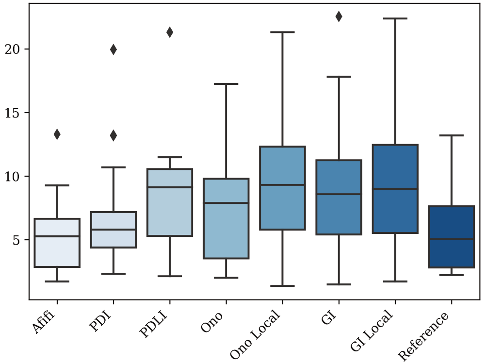
To get the full picture of how well the approach works on our custom evaluation data set, we calculated the
Code
Here is my code, that I wrote for the custom class AfifiRenderer. The first part defines two custom dictionary classes, that prevent us from using the model in a wrong way.
The second part now defines the AfifiRenderer class, that holds the model and the camera pipeline. The render method applies the model to the images and the save method saves the results to disk.
Here is an example how this would be used: